Access the files needed to run this tutorial here
This tutorial is for processing and classifying mercury methylation genes (hgcAB) from a mock community dataset from Gionfriddo et al. 2020. The full-set of paired-end fastq files from the published study can be downloaded from the NCBI SRA database under BioProject: PRJNA608965. A small subset of the mock community dataset is used for this tutorial, ‘mock_community_fastq_tutorial.zip’. The tutorial dataset is only a small subset of the mock community data from the paper. Therefore, there are some differences in data outputs from this tutorial with the results from the full dataset.
The tutorial dataset contains hgcAB amplicon sequencing of two mock communities. Each community is a mix of three cultured Hg-methylator isolates from the Deltaproteobacteria, Methanomicrobia (Euryarchaeota), and Firmicutes. The dataset also includes a salt marsh sediment sample (ID: 1064), and the marsh sample spiked with the two mock communities (1064 + mock community 1, 1064 + mock community 2). The hgcAB genes were amplified with primers ORNL-HgcAB-uni-F, ORNL-HgcAB-uni-32R (Gionfriddo et al. 2020) and sequenced on Illumina Miseq 2×300 bp. The hgcABamplicon is ~980 nt bp long, and therefore with short-read sequencing employed in this study, the forward and reverse reads do not overlap. Only the forward reads are used for downstream analyses. Please see the paper for a more detailed explanation of the methods. The trimmed (201 nt bp) forward read hgcA sequences are classified using the ORNL compiled Hg-methylator database reference package for short sequences, ‘ORNL_HgcA_201.refpkg’.
Before you start:
This tutorial is intended to be run on a Unix/Linux environment. I recommend running Parts 1-4 through a Bioconda environment, which supports 64-bit Linux or Mac OS. The tutorial syntax is written for the versions of programs listed below. If different versions of the programs are used, then some of the command and script syntax may need to be updated. For Parts 1-4 of this tutorial you will need to be able to execute the following programs from the command line:
- Python (version 2.7)
- Trimmomatic (version 0.39)
- Vsearch (version 2.7.0)
- Cd-hit (version 4.6.8)
- Emboss (version 6.5.7)
- Hmmer (version 3.2)
- pplacer (version v1.1.alpha17)
Part 5 of the tutorial utilizes two R scripts to process the taxonomic classifications from the pplacer outputs, and producing a bar plot of relative abundances. You will need to install R (version 3.5.1 or later), and the following R libraries and dependencies:
Part One
Editing raw sequence files, trimming, and quality filtering
- Install python script ‘format_multifile_headers_uparse.py’ & Trimmomatic version 0.39
- Make python script executable:
chmod +x format_multifile_headers_uparse.py
- The tab-delimited text file ‘sample_ids.txt’ has sample IDs and the corresponding fastq files on each line:
SampleID forward_reads.fastq reverse_reads.fastq
- Copy Illumina adapter file ‘NexteraPE-PE.fa’ from Trimmomatic software folder to working directory with fastq files
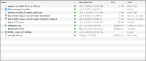
The working directory should look like this:
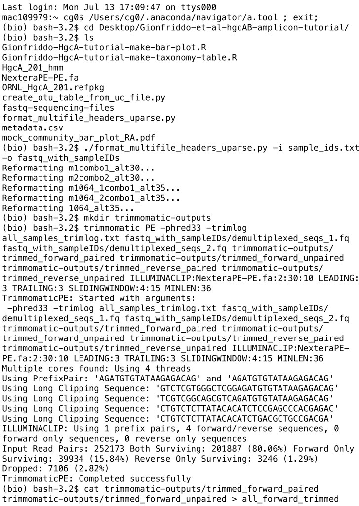
1.1: Reformat read file names with given sample IDs (sample_ids.txt) – will combine all fastq files into single forward (demultiplexed_seqs_1.fq) and reverse (demultiplexed_seqs_2.fq) fastq files into new folder (fastq_with_sampleIDs)
./format_multifile_headers_uparse.py -i sample_ids.txt -o fastq_with_sampleIDs
1.2 Make directory ‘trimmomatic-outputs’
mkdir trimmomatic-outputs
1.3 Trim and quality filter reformatted read files – specify that these are paired-end fastq files with ‘PE’, phred33 refers to format of base quality scores, specify name of log file (samples_trimlog.txt), input fastq files (demultiplexed_seqs_1.fq, demultiplexed_seqs_2.fq), output file names (forward_paired, forward_unpaired, reverse_paired, reverse_unpaired), Illumina adapter and quality filtering parameters (use NexteraPE-PE.fa adapter file), minimum length of reads kept is 36 bp
trimmomatic PE -phred33 -trimlog all_samples_trimlog.txt fastq_with_sampleIDs/demultiplexed_seqs_1.fq fastq_with_sampleIDs/demultiplexed_seqs_2.fq trimmomatic-outputs/trimmed_forward_paired trimmomatic-outputs/trimmed_forward_unpaired trimmomatic-outputs/trimmed_reverse_paired trimmomatic-outputs/trimmed_reverse_unpaired ILLUMINACLIP:NexteraPE-PE.fa:2:30:10 LEADING:3 TRAILING:3 SLIDINGWINDOW:4:15 MINLEN:36
1.4 Since the read sequencing length (2x300bp) was insufficient to fully cover the target sequence length (~1 kbp), and there is no overlap between forward and reverse reads, only forward reads are used for further analysis. Here we combine the forward paired and unpaired reads from the Trimmomatic outputs into one file (all_forward_trimmed) in our working directory
cat trimmomatic-outputs/trimmed_forward_paired trimmomatic-outputs/trimmed_forward_unpaired > all_forward_trimmed
Part Two
Truncate, dereplicate, sort by size, and remove unique sequences prior to clustering reads into OTUs
- Make sure that the output of 1.4, ‘all_forward_trimmed’ is in your working directory
- Install Vsearch (version 2.7.0), Cd-hit (4.6.8), python script create_otu_table_from_uc_file.py
- Make python script executable:
chmod +x create_otu_table_from_uc_file.py
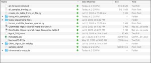
The working directory at the beginning of Part 2 should look like:
2.1 Make new output directory: ‘vsearch-outputs’
mkdir vsearch-outputs
2.2 Truncate reads to same length (201 bp), add suffix ‘_201’ to each read identifier, and get rid of reads that are too short, output is fasta file ‘all_forward_trimmed_201.fa’
vsearch –fastx_filter all_forward_trimmed –fastq_trunclen 201 –label_suffix _201 –fastaout vsearch-outputs/all_forward_trimmed_201.fa
2.3 Dereplicate reads and pull out unique sequences. Relabel remaining sequences ‘Uniq’
vsearch –derep_fulllength vsearch-outputs/all_forward_trimmed_201.fa –strand plus –output vsearch-outputs/all_forward_201_uniques.fa –sizeout –relabel Uniq –fasta_width 0
2.4 Sort by size (i.e. the number of replicates for each sequence) – remove singleton sequences by setting minimum to 2. Identifying unique sequences and removing singleton and replicate sequences helps limit the computational power needed for clustering step.
vsearch –derep_fulllength vsearch-outputs/all_forward_201_uniques.fa –minuniquesize 2 –sizein –sizeout –output vsearch-outputs/all_forward_201_uniques_seqs_sorted.fa –fasta_width 0
2.5 Precluster at 98% prior to Chimera detection – output will be a hits table in uclust format (all.preclustered.uc) and fasta file of centroid representative sequences (all.preclustered.fasta)
vsearch –cluster_size vsearch-outputs/all_forward_201_uniques_seqs_sorted.fa –id 0.98 –strand plus –sizein –sizeout –fasta_width 0 –uc vsearch-outputs/all.preclustered.uc –centroids vsearch-outputs/all.preclustered.fasta
2.6 Search 98% centroid sequences (all.preclustered.fasta) for chimeras using denovo chimera detection – non-chimeric sequences are then saved to fasta file (all.denovo.nonchimeras.fasta)
vsearch –uchime_denovo vsearch-outputs/all.preclustered.fasta –sizein –sizeout –fasta_width 0 –nonchimeras vsearch-outputs/all.denovo.nonchimeras.fasta
2.7 Use cd-hit-est to cluster unique non-chimeric, non-singleton sequences at 90% identity – output will be a fasta file of representative sequences (all.denovo.nonchimeras_cluster90)
cd-hit-est -i vsearch-outputs/all.denovo.nonchimeras.fasta -o vsearch-outputs/all.denovo.nonchimeras_cluster90 -c 0.90 -n 4
2.8 Map original trimmed reads (all_forward_trimmed_201.fa) to representative sequence database (all.denovo.nonchimeras_cluster90) at 90% identity to create hits table in uclust format (all_forward_nonchimeras_cluster90_table.uc). Specify that sequences are in the forward direction with ‘strand plus’. Save OTU table to main working directory.
<p class="has-text-color has-background" style="background-color:#edf0f3;color:#ad5151" value="<amp-fit-text layout="fixed-height" min-font-size="6" max-font-size="72" height="80">vsearch –usearch_global vsearch-outputs/all_forward_trimmed_201.fa –db vsearch-outputs/all.denovo.nonchimeras_cluster90 –id 0.9 –uc all_forward_nonchimeras_cluster90_table.uc –strand plusvsearch –usearch_global vsearch-outputs/all_forward_trimmed_201.fa –db vsearch-outputs/all.denovo.nonchimeras_cluster90 –id 0.9 –uc all_forward_nonchimeras_cluster90_table.uc –strand plus2.9 Convert OTU uclust table to tsv format that can be opened in Excel
./create_otu_table_from_uc_file.py -i all_forward_nonchimeras_cluster90_table.uc -o all_forward_nonchimeras_cluster90_otu
Part Three
Quality filtering centroid representative sequences prior to classification
- Install Emboss (6.5.7), Hmmer (version 3.2)
- Make sure reference package (ORNL_HgcA_201.refpkg) is in working directory
- Make sure hmm reference alignment (HgcA_201_hmm) from reference package (ORNL_HgcA_201.refpkg/HgcA_201_hmm) is in working directory
The working directory at the beginning of Part 3 should look like:

3.1 Make new output directory for hmm-filtering steps: ‘hmm-outputs’
mkdir hmm-outputs
3.2 Translate centroid representative sequences from cd-hit-est output (step 2.6, all.denovo.nonchimeras_cluster90) from nucleotide to amino acid sequences using ‘transeq’ from Emboss package
transeq vsearch-outputs/all.denovo.nonchimeras_cluster90 hmm-outputs/all.denovo.nonchimeras_cluster90_aa
3.3 To filter out centroid sequences that are likely not HgcA or do not begin with the cap-helix region (i.e. the reading frame does not begin on the first base), remove sequences with stop codons by deleting sequences that contain ‘*’
awk ‘/^>/ {printf(“%s%s\t”,(N>0?”\n”:””),$0);N++;next;} {printf(“%s”,$0);} END {printf(“\n”);}’ hmm-outputs/all.denovo.nonchimeras_cluster90_aa | awk -F ‘\t’ ‘!($2 ~ /\*/)’ | tr “\t” “\n” > hmm-outputs/all.denovo.nonchimeras_cluster90_aa_filtered.fa
3.4 Search filtered centroid sequences (all.denovo.nonchimeras_cluster90_aa_filtered.fa) for HgcA sequences using reference HgcA hmm-profile (HgcA_201_hmm) using hmmsearch. Filter out reads that do not align with reference HgcA sequences using an inclusion E-value cutoff of 1E-7. Output will be a table of reads and E values (all.denovo.nonchimeras_cluster90_aa_filtered_hmm_table), text file showing alignment of all centroid sequences with reference HgcA and E-values (all.denovo.nonchimeras_cluster90_aa_filtered_hmm_output) and alignment of centroid sequences that passed inclusion threshold with reference sequences (all.denovo.nonchimeras_cluster90_aa_filtered_hmm_alignment)
hmmsearch –tblout hmm-outputs/all.denovo.nonchimeras_cluster90_aa_filtered_hmm_table -o hmm-outputs/all.denovo.nonchimeras_cluster90_aa_filtered_hmm_output –incE 1E-7 -A hmm-outputs/all.denovo.nonchimeras_cluster90_aa_filtered_hmm_alignment HgcA_201_hmm hmm-outputs/all.denovo.nonchimeras_cluster90_aa_filtered.fa
3.5 Align filtered centroid sequences from step 3.2 (all.denovo.nonchimeras_cluster90_aa_filtered_hmm_alignment) to stockhold formatted alignment of reference sequences in reference package (ORNL_HgcA_201.refpkg/aa_201bp_ref_alignment_stockholm.stockholm) using hmm model (HgcA_201_hmm) produing a Stockholm formatted alignment of filtered centroid sequences and reference sequences (all.denovo.nonchimeras_cluster90_aa_filtered_hmm_alignment.sto) that can be used for classification
hmmalign -o hmm-outputs/all.denovo.nonchimeras_cluster90_aa_filtered_hmm_alignment.sto –mapali ORNL_HgcA_201.refpkg/aa_201bp_ref_alignment_stockholm.stockholm HgcA_201_hmm hmm-outputs/all.denovo.nonchimeras_cluster90_aa_filtered_hmm_alignment
Part Four
Classify centroid HgcA sequences based on phylogenetic placement
- Install pplacer (v1.1.alpha17-6-g5cecf99)
- Make sure the ORNL HgcA reference package is in the into working directory (ORNL_HgcA_201.refpkg)
The working directory at the beginning of Part 4 should look like:

4.1 Place aligned centroid sequences (all.denovo.nonchimeras_cluster90_aa_filtered_hmm_alignment.sto) onto maximum likelihood reference HgcA tree in reference package (HgcA_201.refpkg). Specify to calculate posterior probabilities based on alignment of query sequence with reference sequence (-p), specify that the maximum number of placements to keep is one (–keep-at-most 1), set the maximum branch length to 1 (–max-pend 1) (this ensures that sequences that are highly dissimilar to HgcA are not placed on the tree – this is the last filtering step for identifying non-HgcA sequences). Output will be a jplace file containing reads placed on max-like tree (all.denovo.nonchimeras_cluster90_aa_filtered_hmm_alignment.jplace)
pplacer -p –keep-at-most 1 –max-pend 1 -c ORNL_HgcA_201.refpkg/ hmm-outputs/all.denovo.nonchimeras_cluster90_aa_filtered_hmm_alignment.sto
4.2 Make a sqlite database for classifications (all_forward_nonchimeric_90_201_classify)
rppr prep_db –sqlite all_forward_nonchimeric_90_201_classify -c ORNL_HgcA_201.refpkg/
4.3 Assign taxonomy to reads based on where the query sequences have been placed on reference tree (all.denovo.nonchimeras_cluster90_aa_filtered_hmm_alignment.jplace), uses posterior probability (–pp) and lowest common ancestor of branch to classify, and uses a 90% confidence cut-off for identification as default. Writes classifications to the sqlite database made in step 4.2 (all_forward_nonchimeric_90_201_classify).
guppy classify -c ORNL_HgcA_201.refpkg/ –pp –sqlite all_forward_nonchimeric_90_201_classify all.denovo.nonchimeras_cluster90_aa_filtered_hmm_alignment.jplace
4.4 To write guppy classifications to csv file:
guppy to_csv –point-mass –pp -o all.denovo.nonchimeras_cluster90_classifications.csvall.denovo.nonchimeras_cluster90_aa_filtered_hmm_alignment.jplace
4.5 To make a visualization showing placements on reference tree:
guppy tog –pp -o all.denovo.nonchimeras_cluster90_classifications.nwkall.denovo.nonchimeras_cluster90_aa_filtered_hmm_alignment.jplace
4.6 The saved terminal output from Parts 1-4 can be found at the end of this document
Part Five
Visualizing the classifications and relative abundance of OTUs using R
The OTU table and pplacer objects are inputed into R in order to process the taxonomy classifications, calculate relative abundances of OTUs for each sample, and create a visualization of the data. To run the R scripts included in this tutorial (shown below, Gionfriddo-HgcA-tutorial-make-taxonomy-table.R and Gionfriddo-HgcA-tutorial-make-bar-plot.R), you will need to install R (version 3.5.1 or later), and the R libraries BoSSA, phyloseq, ggplot2, RColorBrewer.
Before running the scripts, double check that the working directory contains the pplacer outputs, the OTU table output (all_forward_nonchimeras_cluster90_otu), the metadata file for the mock community dataset (metadata.csv), and the reference package (ORNL_HgcA_201.refpkg).
The working directory should look like this:

5.1 The R script ‘Gionfriddo-HgcA-tutorial-make-taxonomy-table.R’ assigns taxonomy to OTUs using the phylogenetic placements and classifications assigned using pplacer. Make sure the path to the working directory in the R script is indeed the path to the tutorial folder on your computer. Currently it is set to ‘~/Desktop/Gionfriddo-et-al-hgcAB-amplicon-tutorial’
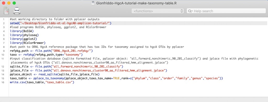
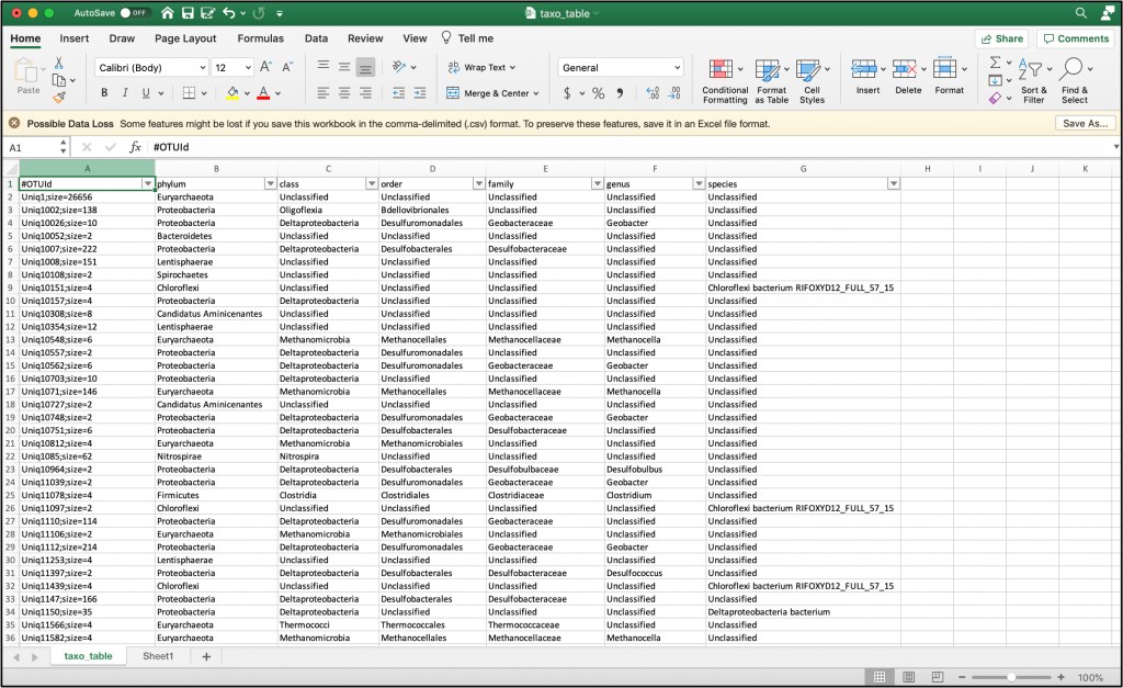
5.2 The output from the R script will be a table, ‘taxo_table.csv’, with OTU Ids, and taxonomy information. Label the first column ‘#OTUId’

5.3 Edit the OTU IDs to remove the ‘_1/1-67’, ‘_1/1-62’, etc. at the end of the IDs. The format of the IDs need to match the OTU table (‘all_forward_nonchimeras_cluster90_otu’)
5.4 Using the OTU IDs from the taxonomy table, filter the OTU table ‘all_forward_nonchimeras_cluster90_otu’ for only those that passed classification guidelines and were identified as HgcA. Copy the OTU IDs from ‘taxo_table.csv’, and paste below the OTU IDs in the OTU table, then use ‘highlight duplicate cells’ conditional formatting in Excel. Then filter to view only highlighted cells, copy the filtered OTU table to new Excel spreadsheet, and save as a csv-file, ‘otu_table_filtered.csv’

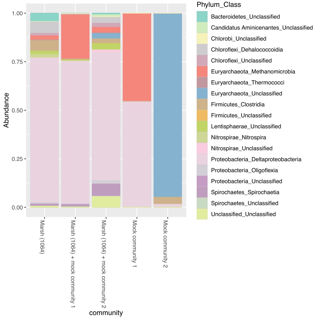
5.5 The R script ‘Gionfriddo-HgcA-tutorial-make-bar-plot.R’ inputs the OTU table ‘otu_table_filtered.csv’ and taxonomy table ‘taxo_table.csv’, transforms the OTU counts as relative abundances for each sample, and creates a bar plot of the relative abundance of each OTU. The bar plot colors correspond to phylum and class of each OTU.
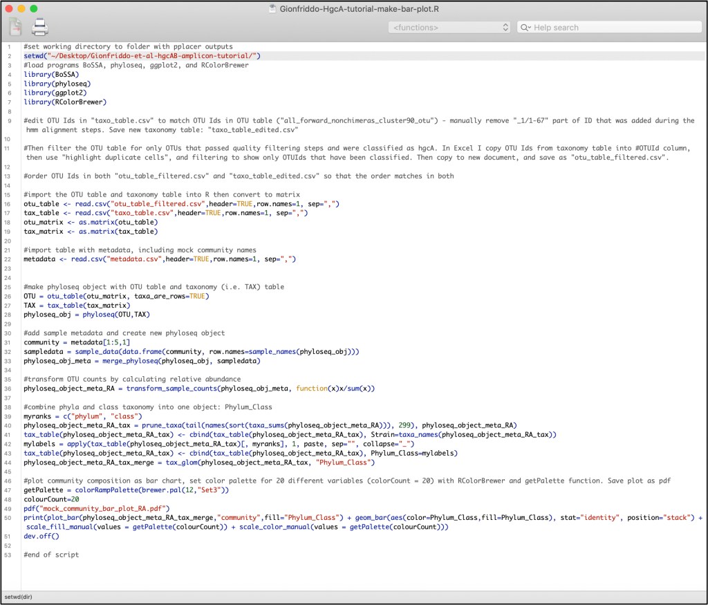
5.6 The output of the R script is a bar plot (mock_community_bar_plot_RA.pdf) of the relative abundance of HgcA OTUs for the Marsh community (1064), two mock communities, and marsh sample spiked with the two marsh communities. The bars are colored by the phylum and class assigned to each OTU.
Terminal Outputs from Parts 1-4